Flexibility under Uncertainty

The previous chapter only modelled a single scenario where flexibility was employed. In this chapter, we follow [dNG18] (Chapter 9) in assessing how flexibility can be used to manage, and benefit from, uncertainty.

Multiple Market Scenarios

If we can produce one future market scenario, we can also produce many. To incorporate our uncertainty about how future scenarios may unfold, we derive Market input parameters by sampling from probability distributions that we suspect are realistic for the market in question.

Market Parameters from Sampling Distributions of their Likelihoods

Rangekeeper provides alternate methods for Market dynamics modules that take probability distributions as inputs, rather than single values. These methods also require us to specify how many iterations (runs, or simulations) we will produce.

Begin with importing required libraries and configuring our context:

import locale
import warnings
warnings.simplefilter(action='ignore', category=FutureWarning) # to suppress pandas warnings about deprecated functions

import pandas as pd
import seaborn as sns

import rangekeeper as rk

locale.setlocale(locale.LC_ALL, 'en_AU')
units = rk.measure.Index.registry
currency = rk.measure.register_currency(registry=units)

Specify how many iterations (scenarios) we will produce. This matches the number of samples we will take from the probability distributions:

iterations = 2000

We also need to define the overall Span of the Market:

frequency = rk.duration.Type.YEAR
num_periods = 25
span = rk.span.Span.from_duration(
    name="Span",
    date=pd.Timestamp(2000, 1, 1),
    duration=frequency,
    amount=num_periods)
sequence = span.to_sequence(frequency=frequency)

Overall Trend

Following how [dNG18] construct market simulations, a Rangekeeper Market Trend can sample from distributions defining the growth rate (trend) and initial rent value.

For initial (rent) value, typically values would not be more than 0.05 or 0.1, at most. Initial rents should be able to be estimated pretty accurately in the realistic pro-forma, especially for existing buildings.

The growth rate distribution reflects uncertainty in the long-run trend growth rate (that applies throughout the entire scenario. In [dNG18], this is modeled as a triangular distribution (though Rangekeeper provides other distributions easily), and the half-range should typically be a small value, at most .01 or .02, unless there is great uncertainty in the long-run average growth rate in the economy (such as perhaps in some emerging market countries), or if one is modeling nominal values and there is great uncertainty about what the future rate of inflation will be (but in such cases it is better to model real values, net of inflation anyway).

(From [dNG18], accompanying Excel spreadsheets)

First we define the distributions:

growth_rate_dist = rk.distribution.Symmetric(
    type=rk.distribution.Type.TRIANGULAR,
    mean=-.0005,
    residual=.005)
initial_value_dist = rk.distribution.Symmetric(
    type=rk.distribution.Type.TRIANGULAR,
    mean=.05,
    residual=.005)

We now produce the resultant Trends:

cap_rate = .05

trends = rk.dynamics.trend.Trend.from_likelihoods(
    sequence=sequence,
    cap_rate=cap_rate,
    growth_rate_dist=growth_rate_dist,
    initial_value_dist=initial_value_dist,
    iterations=iterations)

We can check that the Trends have been produced as expected:

initial_values = [trend.initial_value for trend in trends]
sns.histplot(
    data=initial_values,
    bins=20,
    kde=True)

<Axes: ylabel='Count'>

Volatility

Volatility inputs do not require sampling from distributions, but we will be producing multiple Volatility objects, one for each Trend:

volatility_per_period = .1
autoregression_param = .2
mean_reversion_param = .3

volatilities = rk.dynamics.volatility.Volatility.from_trends(
    sequence=sequence,
    trends=trends,
    volatility_per_period=volatility_per_period,
    autoregression_param=autoregression_param,
    mean_reversion_param=mean_reversion_param)

Cyclicality

[dNG18] document multiple means to incorporate estimations of market cycle parameters into a market simulation. Here we replicate the distribution parameters for use in Rangekeeper.

We are agnostic about where the market currently is in the cycle, and want to simulate all possibilities; thus the Space (Rent) Cycle Phase Proportion (of its period) is sampled from a uniform distribution defaulted to a range between 0 & 1):

space_cycle_phase_prop_dist = rk.distribution.Uniform()

The Space (Rent) Cycle Period is a random sample between 10 & 20 years:

space_cycle_period_dist=rk.distribution.Symmetric(
    type=rk.distribution.Type.UNIFORM,
    mean=15,
    residual=5)

The Space (Rent) Cycle peak-to-trough Height is set at 50% (see residual fixed to 0):

space_cycle_height_dist=rk.distribution.Symmetric(
    type=rk.distribution.Type.UNIFORM,
    mean=.5,
    residual=0)

The Asset (Cap Rate) Cycle Phase differs from the Space Cycle by between -1/10th and 1/10th of the Space Cycle Period:

asset_cycle_phase_diff_prop_dist=rk.distribution.Symmetric(
    type=rk.distribution.Type.UNIFORM,
    mean=0,
    residual=.1)

The Asset (Cap Rate) Cycle Period in between -1 and 1 year different to that of the Space (Rent) Cycle’s

asset_cycle_period_diff_dist=rk.distribution.Symmetric(
    type=rk.distribution.Type.UNIFORM,
    mean=0,
    residual=1)

The Asset (Cap Rate) Cycle Amplitude is fixed to 2%:

asset_cycle_amplitude_dist=rk.distribution.Symmetric(
    type=rk.distribution.Type.UNIFORM,
    mean=.02,
    residual=0.)

For both the Space and Asset Cycles, we remove any cycle asymmetries, in order to align with [dNG18]’s spreadsheet for Chapters 8, 9, 10. In future classes (and possibly future editions), they incorporate cycle asymmetries.

space_cycle_asymmetric_parameter_dist=rk.distribution.Symmetric(
    type=rk.distribution.Type.UNIFORM,
    mean=0,
    residual=0.)
asset_cycle_asymmetric_parameter_dist=rk.distribution.Symmetric(
    type=rk.distribution.Type.UNIFORM,
    mean=0,
    residual=0.)

We now produce the resultant Cycles:

cyclicalities = rk.dynamics.cyclicality.Cyclicality.from_likelihoods(
    sequence=sequence,
    space_cycle_phase_prop_dist=space_cycle_phase_prop_dist,
    space_cycle_period_dist=space_cycle_period_dist,
    space_cycle_height_dist=space_cycle_height_dist,
    asset_cycle_phase_diff_prop_dist=asset_cycle_phase_diff_prop_dist,
    asset_cycle_period_diff_dist=asset_cycle_period_diff_dist,
    asset_cycle_amplitude_dist=asset_cycle_amplitude_dist,
    space_cycle_asymmetric_parameter_dist=space_cycle_asymmetric_parameter_dist,
    asset_cycle_asymmetric_parameter_dist=asset_cycle_asymmetric_parameter_dist,
    iterations=iterations)

Noise & Black Swan

Noise & Black Swan inputs do not require sampling from distributions:

noise = rk.dynamics.noise.Noise(
    sequence=sequence,
    noise_dist=rk.distribution.Symmetric(
        type=rk.distribution.Type.TRIANGULAR,
        mean=0.,
        residual=.1))
black_swan = rk.dynamics.black_swan.BlackSwan(
    sequence=sequence,
    likelihood=.05,
    dissipation_rate=mean_reversion_param,
    probability=rk.distribution.Uniform(),
    impact=-.25)

Markets

Now we can integrate the previous constructs into multiple Market simulations:

markets = rk.dynamics.market.Market.from_likelihoods(
    sequence=sequence,
    trends=trends,
    volatilities=volatilities,
    cyclicalities=cyclicalities,
    noise=noise,
    black_swan=black_swan)

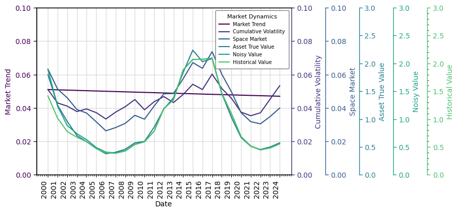
As an example, here is one of the Markets (drawn from the markets by a random integer):

import random
sample_market = markets[random.Random(0).randint(0, iterations - 1)]
table = rk.flux.Stream(
    name='Market Dynamics',
    flows=[
        sample_market.trend,
        sample_market.volatility.volatility,
        sample_market.volatility.autoregressive_returns,
        sample_market.volatility,
        sample_market.cyclicality.space_waveform,
        sample_market.space_market,
        sample_market.cyclicality.asset_waveform,
        sample_market.asset_market,
        sample_market.asset_true_value,
        sample_market.space_market_price_factors,
        sample_market.noisy_value,
        sample_market.historical_value,
        sample_market.implied_rev_cap_rate,
        sample_market.returns
        ],
    frequency=frequency)
table.plot(
        flows={
            'Market Trend': (0, .1),
            'Cumulative Volatility': (0, .1),
            'Space Market': (0, .1),
            'Asset True Value': (0, 3),
            'Noisy Value': (0, 3),
            'Historical Value': (0, 3)
            }
    )

Comparing Models

From [dNG18]: to obtain the value of flexibility, we compare the project utilizing flexibility against a base case or alternative that lacks the particular flexibility or rule we are evaluating. We must expose the inflexible case to the same independent, random future scenarios as the flexible case. We must compute the outcomes for the two cases, inflexible and flexible, under exactly the same scenarios of pricing factor realizations. We can then compare the results of both the inflexible and flexible cases, not only against the (single‐number) traditional pro forma metrics, but also side by side against each other for the entire distribution of possible (ex‐post) outcomes, recognizing the uncertainty and price dynamics that realistically exist.

Inflexible (Base) Model

Define the Base Model as we did the Ex-Post Inflexible Model in the previous section:

params = {
    'start_date': pd.Timestamp('2001-01-01'),
    'num_periods': 10,
    'frequency': rk.duration.Type.YEAR,
    'acquisition_cost': -1000 * currency.units,
    'initial_income': 100 * currency.units,
    'growth_rate': 0.02,
    'vacancy_rate': 0.05,
    'opex_pgi_ratio': 0.35,
    'capex_pgi_ratio': 0.1,
    'exit_caprate': 0.05,
    'discount_rate': 0.07
    }

Show code cell source Hide code cell source

class BaseModel:
    def __init__(self) -> None:
        pass
    def set_params(self, params: dict) -> None:
        self.params = params
    def set_market(self, market: rk.dynamics.market.Market) -> None:
        self.market = market
    def init_spans(self):
        self.calc_span = rk.span.Span.from_duration(
            name='Span to Calculate Reversion',
            date=self.params['start_date'],
            duration=self.params['frequency'],
            amount=self.params['num_periods'] + 1)
        self.acq_span = rk.span.Span.from_duration(
            name='Acquisition Span',
            date=rk.duration.offset(
                date=self.params['start_date'],
                amount=-1,
                duration=self.params['frequency']),
            duration=self.params['frequency'])
        self.span = self.calc_span.shift(
            name='Span',
            amount=-1,
            duration=self.params['frequency'])
        self.reversion_span = self.span.shift(
            name='Reversion Span',
            amount=self.params['num_periods'] - 1,
            duration=self.params['frequency'],
            bound='start')
    def calc_acquisition(self):
        self.acquisition = rk.flux.Flow.from_projection(
            name='Acquisition',
            value=self.params['acquisition_cost'],
            proj=rk.projection.Distribution(
                form=rk.distribution.Uniform(),
                sequence=self.acq_span.to_sequence(frequency=self.params['frequency'])),
            units=currency.units)
    def calc_egi(self):
        pgi = rk.flux.Flow.from_projection(
            name='Potential Gross Income',
            value=self.params['initial_income'],
            proj=rk.projection.Extrapolation(
                form=rk.extrapolation.Compounding(
                    rate=self.params['growth_rate']),
                sequence=self.calc_span.to_sequence(frequency=self.params['frequency'])),
            units=currency.units)

        # Construct a Stream that multiplies the Base Model's PGI by the
        # simulated Market's Space Market factors
        self.pgi = (rk.flux.Stream(
            name='Potential Gross Income',
            flows=[
                pgi,
                self.market.space_market_price_factors.trim_to_span(self.calc_span)
                ],
            frequency=self.params['frequency'])
                .product(registry=rk.measure.Index.registry))

        self.vacancy = rk.flux.Flow(
            name='Vacancy Allowance',
            movements=self.pgi.movements * -self.params['vacancy_rate'],
            units=currency.units)
        self.egi = (rk.flux.Stream(
            name='Effective Gross Income',
            flows=[self.pgi, self.vacancy],
            frequency=self.params['frequency'])
                .sum())
    def calc_noi(self):
        self.opex = (rk.flux.Flow(
            name='Operating Expenses',
            movements=self.pgi.movements * self.params['opex_pgi_ratio'],
            units=currency.units)
                .invert())
        self.noi = (rk.flux.Stream(
            name='Net Operating Income',
            flows=[self.egi, self.opex],
            frequency=self.params['frequency'])
                .sum())
    def calc_ncf(self):
        self.capex = (rk.flux.Flow(
            name='Capital Expenditures',
            movements=self.pgi.movements * self.params['capex_pgi_ratio'],
            units=currency.units)
                .invert())
        self.net_cf = (rk.flux.Stream(
            name='Net Annual Cashflow',
            flows=[self.noi, self.capex],
            frequency=self.params['frequency'])
                .sum())
    def calc_reversion(self):
            # Construct the Reversions using the simulated Market's Asset Market
            # factors (cap rates):
            self.reversions = (rk.flux.Flow(
                name='Reversions',
                movements=self.net_cf.movements.shift(periods=-1).dropna() /
                          self.market.implied_rev_cap_rate.movements,
                units=currency.units)
                    .trim_to_span(span=self.span))

            self.reversion = self.reversions.trim_to_span(
                span=self.reversion_span,
                name='Reversion')
            self.pbtcfs = rk.flux.Stream(
                name='PBTCFs',
                flows=[
                    self.net_cf.trim_to_span(span=self.span),
                    self.reversions.trim_to_span(span=self.reversion_span)
                    ],
                frequency=self.params['frequency'])
    def calc_metrics(self):
        pvs = []
        irrs = []
        for period in self.net_cf.trim_to_span(span=self.span).movements.index:
            cumulative_net_cf = self.net_cf.trim_to_span(
                span=rk.span.Span(
                    name='Cumulative Net Cashflow Span',
                    start_date=self.params['start_date'],
                    end_date=period))
            reversion = rk.flux.Flow(
                movements=self.reversions.movements.loc[[period]],
                units=currency.units)
            cumulative_net_cf_with_rev = rk.flux.Stream(
                name='Net Cashflow with Reversion',
                flows=[
                    cumulative_net_cf,
                    reversion
                    ],
                frequency=self.params['frequency'])
            pv = cumulative_net_cf_with_rev.sum().pv(
                name='Present Value',
                frequency=self.params['frequency'],
                rate=self.params['discount_rate'])
            pvs.append(pv.collapse().movements)

            incl_acq = rk.flux.Stream(
                name='Net Cashflow with Reversion and Acquisition',
                flows=[cumulative_net_cf_with_rev.sum(), self.acquisition],
                frequency=self.params['frequency'])

            irrs.append(round(incl_acq.sum().xirr(), 4))

        self.pvs = rk.flux.Flow(
            name='Present Values',
            movements=pd.concat(pvs),
            units=currency.units)
        self.irrs = rk.flux.Flow(
            name='Internal Rates of Return',
            movements=pd.Series(irrs, index=self.pvs.movements.index),
            units=None)
    def generate(self):
        self.init_spans()
        self.calc_acquisition()
        self.calc_egi()
        self.calc_noi()
        self.calc_ncf()
        self.calc_reversion()
        self.calc_metrics()

For each Market, we then run the Base Model. To speed this up we can use multiprocessing, so we need to import and configure a few libraries:

import os
from typing import List
import multiprocess
import pint
pint.set_application_registry(rk.measure.Index.registry)

inflex_scenarios = []
for market in markets:
    scenario = BaseModel()
    scenario.set_params(params.copy())
    scenario.set_market(market)
    inflex_scenarios.append(scenario)

def generate(scenario):
    scenario.generate()
    return scenario
inflex_scenarios = multiprocess.Pool(os.cpu_count()).map(
    generate,
    inflex_scenarios)

Flexible Model

Similarly, we set up the Flexible Model with our Policy:

def exceed_pricing_factor(state: rk.flux.Flow) -> List[bool]:
    threshold = 1.2
    result = []
    for i in range(state.movements.index.size):
        if any(result):
            result.append(False)
        else:
            if i < 1:
                result.append(False)
            else:
                if state.movements.iloc[i] > threshold:
                    result.append(True)
                else:
                    result.append(False)
    return result

def adjust_hold_period(
        model: object,
        decisions: List[bool]) -> object:
    # Get the index of the decision flag:
    try:
        idx = decisions.index(True)
    except ValueError:
        idx = len(decisions)

    # Adjust the Model's holding period:
    policy_params = model.params.copy()
    policy_params['num_periods'] = idx

    # Re-run the Model with updated params:
    model.set_params(policy_params)
    model.generate()
    return model

stop_gain_resale_policy = rk.policy.Policy(
    condition=exceed_pricing_factor,
    action=adjust_hold_period)

And we run the Flexible Model for each Market:

policy_args = [(scenario.market.space_market_price_factors, scenario) for scenario in inflex_scenarios]
flex_scenarios = multiprocess.Pool(os.cpu_count()).map(
    stop_gain_resale_policy.execute,
    policy_args)

Results

We can now compare the results of the Base and Flexible Models with some descriptive statistics

import scipy.stats as ss

Time 0 Present Values at OCC

inflex_pvs = pd.Series([scenario.pvs.movements.iloc[-1] for scenario in inflex_scenarios])
flex_pvs = pd.Series([scenario.pvs.movements.iloc[-1] for scenario in flex_scenarios])
diff_pvs = flex_pvs - inflex_pvs

pvs = pd.DataFrame({
    'Inflexible': inflex_pvs,
    'Flexible': flex_pvs,
    'Difference': diff_pvs})
pvs.describe()

	Inflexible	Flexible	Difference
count	2000.000000	2000.000000	2000.000000
mean	1077.276022	1471.823622	394.547600
std	346.825710	409.756527	571.287343
min	529.877313	519.892437	-1196.914766
25%	798.547972	1220.486400	-7.520586
50%	979.035364	1487.301431	388.425044
75%	1315.903294	1755.160225	829.231786
max	2358.785044	2445.322698	1750.762120

At a high level, we can see from the mean and median (50th percentile) results that the Flexible Model produces a higher PV than the Inflexible Model (by about $400. However, there still is a significant distortion of the distributions from normal, as can be seen in the skewness and kurtosis statistics.

pvs.skew()

Inflexible    0.828175
Flexible     -0.281891
Difference   -0.077777
dtype: float64

pvs.kurtosis()

Inflexible    0.039147
Flexible     -0.146919
Difference   -0.658811
dtype: float64

print('PV Diffs t-stat: \n{}'.format(
    ss.ttest_1samp(diff_pvs, 0)))

PV Diffs t-stat: 
TtestResult(statistic=30.885867334080228, pvalue=1.379607479805352e-171, df=1999)

PVs Cumulative Distribution (‘Target Curves’)

To get a better idea of just how the Flexible Model outperforms the Inflexible Model, we can plot their distributions of outcomes

Present Values

sns.histplot(
    data=pvs.drop(columns=['Difference']),
    binwidth=50,
    kde=True
    )

<Axes: ylabel='Count'>

To make reading the plot easier and identify just how and when the Flexible model outperforms the Inflexible, we can also plot the cumulative distribution of the PVs:

sns.ecdfplot(
    data=pvs.drop(columns=['Difference']))

<Axes: ylabel='Proportion'>

Realized IRR at Market Value Price

inflex_irrs = pd.Series([scenario.irrs.movements.iloc[-1] for scenario in inflex_scenarios])
flex_irrs = pd.Series([scenario.irrs.movements.iloc[-1] for scenario in flex_scenarios])
diff_irrs = flex_irrs - inflex_irrs

irrs = pd.DataFrame({
    'Inflexible': inflex_irrs,
    'Flexible': flex_irrs,
    'Difference': diff_irrs})
irrs.describe()

	Inflexible	Flexible	Difference
count	2000.000000	2000.00000	2000.000000
mean	0.071688	0.30250	0.230812
std	0.040480	0.36309	0.376362
min	-0.018500	-0.04190	-0.171800
25%	0.038900	0.09465	0.002300
50%	0.067350	0.13920	0.059350
75%	0.104975	0.31485	0.270175
max	0.177400	1.61650	1.599500

irrs.skew()

Inflexible    0.202274
Flexible      1.879735
Difference    1.807136
dtype: float64

irrs.kurtosis()

Inflexible   -0.889110
Flexible      2.462491
Difference    2.229461
dtype: float64

print('IRR Diffs t-stat: \n{}'.format(
    ss.ttest_1samp(diff_irrs, 0)))

IRR Diffs t-stat: 
TtestResult(statistic=27.42634134595045, pvalue=7.795094497078348e-141, df=1999)

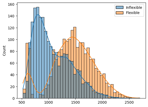
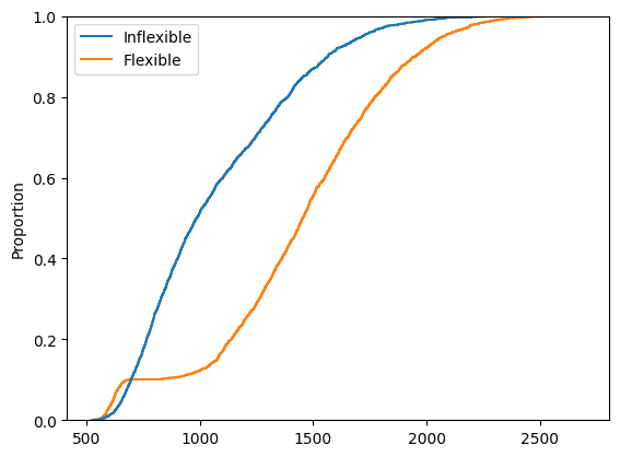
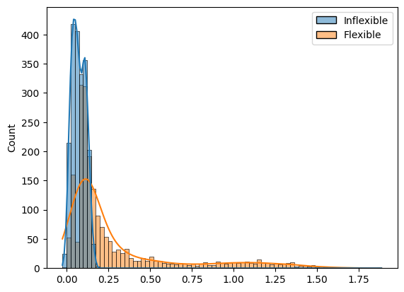
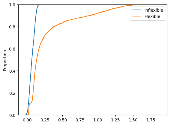
IRRs Cumulative Distribution (‘Target Curves’)

g = sns.histplot(
    data=irrs.drop(columns=['Difference']),
    binwidth=.025,
    kde=True
    )

sns.ecdfplot(
    data=irrs.drop(columns=['Difference']))

<Axes: ylabel='Proportion'>

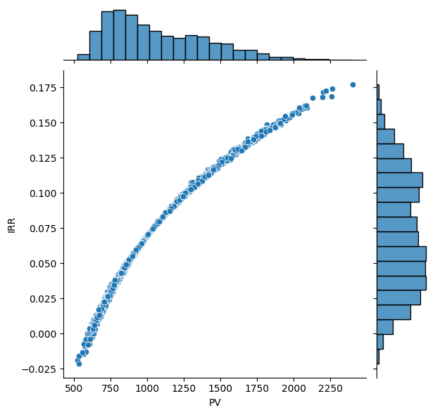
IRRs x PVs

Inflexible Model

inflex_irr_x_pv = pd.DataFrame({
    'PV': inflex_pvs,
    'IRR': inflex_irrs,})
sns.jointplot(
    data=inflex_irr_x_pv,
    x='PV',
    y='IRR',
    kind='scatter')

<seaborn.axisgrid.JointGrid at 0x32a007950>

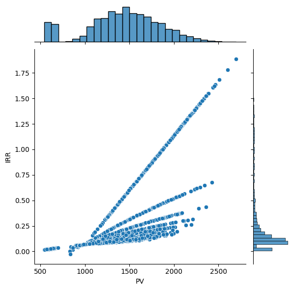
Flexible Model

flex_irr_x_pv = pd.DataFrame({
    'PV': flex_pvs,
    'IRR': flex_irrs})
sns.jointplot(
    data=flex_irr_x_pv,
    x='PV',
    y='IRR',
    kind='scatter')

<seaborn.axisgrid.JointGrid at 0x32a009ad0>

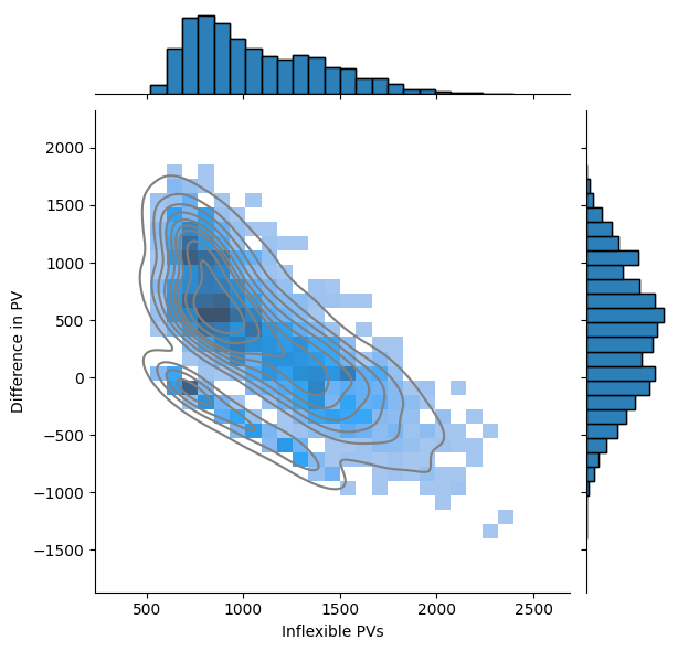
PVs Diffs

PV Difference as a function of Inflex PV

diff_pvs_x_inflex_pvs = pd.DataFrame({
    'Inflexible PVs': inflex_pvs,
    'Difference in PV': diff_pvs})
g = sns.jointplot(
    data=diff_pvs_x_inflex_pvs,
    x='Inflexible PVs',
    y='Difference in PV',
    kind='hist')
g.plot_joint(
    sns.kdeplot,
    color='grey',
    zorder=1,
    levels=10)
g.plot_marginals(
    sns.histplot
    )

<seaborn.axisgrid.JointGrid at 0x32a185450>

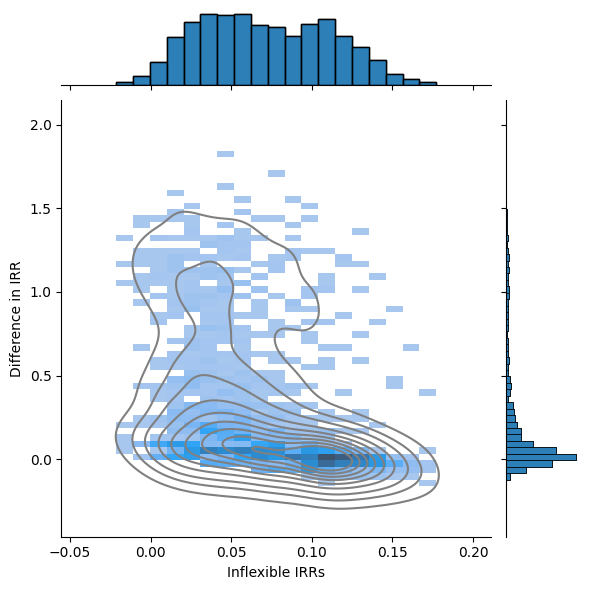
IRR Difference as a function of Inflex IRR

diff_irrs_x_inflex_irrs = pd.DataFrame({
    'Inflexible IRRs': inflex_irrs,
    'Difference in IRR': diff_irrs})
g = sns.jointplot(
    data=diff_irrs_x_inflex_irrs,
    x='Inflexible IRRs',
    y='Difference in IRR',
    kind='hist')
g.plot_joint(
    sns.kdeplot,
    color='grey',
    zorder=1,
    levels=10)
g.plot_marginals(
    sns.histplot
    )

<seaborn.axisgrid.JointGrid at 0x32a3c3fd0>