A Basic Discounted Cash Flow Valuation#
Chapter 1 of [dNG18] showcases the structure and functionality of a basic Discounted Cash Flow (DCF) Valuation for a real estate property.
Like in the vast majority of cases, the implementation of their DCF model is in Microsoft Excel. However, in these notebooks, we will be implementing the same methodology in Python, using the Rangekeeper open source library.
In this notebook, the core computational objects (classes), their functionality, and how they are composed together into a valuation model are outlined.
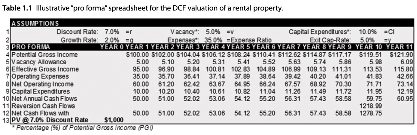
To do so, we will be replicating Table 1.1 from [dNG18], which describes this DCF:
First, we will need to import any neccesary libraries, as well as the
Rangekeeper library, that we alias to rk:
Import Libraries:
import locale
import pandas as pd

# Import Rangekeeper:
import rangekeeper as rk
The Foundational Elements of a Proforma#
A Flow#
The core element of a Cash Flow analysis is the cash flow itself; a sequence of ‘movements’ of currency (whether positive – inflow, or negative – outflow) , where each movement is associated with a date and a quantity. A movement could be considered a transaction, payment, or transfer of currency, but it does not consider the parties involved – only its amount, date, and direction.
A cash flow is also sometimes referred to as a ‘line item’, which is a way of designating the subject of flows, e.g.: “Operational Expenses”, or “Income from Building 2’s Parking”
A cash flow is implemented in Rangekeeper as a Flow object (from the flux
module), which uses a pandas Series
object to encapsulate the movements of a quantity (with specified units, like
currency, energy, mass, etc.) that occur at specified dates.
Note: the Flow’s movements Series index is a Pandas DatetimeIndex, and its values are floats.
Initializing a Flow#
First we initialize the currency used in our Proforma. Currencies are a type of
Measure, which encapsulate Pint unit
definitions. Rangekeeper uses the standard library’s locale module to set
the currency units.
locale.setlocale(locale.LC_ALL, 'en_AU')
units = rk.measure.Index.registry
currency = rk.measure.register_currency(registry=units)
print(currency)
Rangekeeper Measure: "Australian Dollar". Currency of ['AUSTRALIA', 'COCOS (KEELING) ISLANDS', 'CHRISTMAS ISLAND', 'HEARD & MCDONALD ISLANDS', 'KIRIBATI', 'NORFOLK ISLAND', 'NAURU', 'TUVALU']. Units: AUD
Next we define a Flow object from a list of dates and amounts:
transactions = {
    pd.Timestamp('2020-01-01'): 100,
    pd.Timestamp('2020-01-02'): 200,
    pd.Timestamp('2019-01-01'): 300,
    pd.Timestamp('2020-12-31'): -100
    }

movements = pd.Series(data=transactions)

cash_flow = rk.flux.Flow(
    name='Operational Expenses',
    movements=movements,
    units=currency.units)
We can view the object we just created by simply calling it:
cash_flow
| Operational Expenses | |
|---|---|
| 2020-01-01 00:00:00 | $100.00 |
| 2020-01-02 00:00:00 | $200.00 |
| 2019-01-01 00:00:00 | $300.00 |
| 2020-12-31 00:00:00 | -$100.00 |
We can also inspect it by displaying its ‘movements’ (a Pandas Series), and its
index (the Pandas Series’ DateTimeIndex):
cash_flow.movements
2020-01-01    100.0
2020-01-02    200.0
2019-01-01    300.0
2020-12-31   -100.0
Name: Operational Expenses, dtype: float64
cash_flow.movements.index
DatetimeIndex(['2020-01-01', '2020-01-02', '2019-01-01', '2020-12-31'], dtype='datetime64[ns]', freq=None)
It’s units can be inspected by calling its units property:
cash_flow.units
Overview of a Flow#
As you can see, a Flow has three properties:
it’s Name,
a Pandas Series of date-stamped amounts (‘Movements’), and
the units of the movement’s amounts
Note the following:
The movements can be in any (temporal) order,
The movements can be positive or negative,
The movements will be (or converted to)
floatsThe pd.Series index is a pd.DatetimeIndex
All this information can be inspected via the display() method:
cash_flow.display()
Name: Operational Expenses
Units: AUD
Movements:
|                     |   Operational Expenses |
|---------------------|------------------------|
| 2020-01-01 00:00:00 |                $100.00 |
| 2020-01-02 00:00:00 |                $200.00 |
| 2019-01-01 00:00:00 |                $300.00 |
| 2020-12-31 00:00:00 |               -$100.00 |
A Span#
Spans are used to define intervals of time that encompass the movements of a
Flow.
A Span is a pd.Interval of pd.Timestamps that bound its start and end dates.
# Define a Span:
start_date = pd.Timestamp('2001-01-01')
num_periods = 11
span = rk.duration.Span.from_duration(
    name='Operation',
    date=start_date,
    duration=rk.duration.Type.YEAR,
    amount=num_periods)
print(span)
Span: Operation
Start Date: 2001-01-01
End Date: 2011-12-31
A Projection#
A Projection takes a value and casts it over a sequence of periods according
to a specified logic. There are two classes of the form of the logic:
Extrapolation, which takes a starting value and from it generates a sequence of values over a sequence of dates, and
Distribution, which takes a total value and subdivides it over a sequence of dates.
To match the logic of line 4, ‘Potential Gross Income’, in Table 1.1 above, we will use a “Compounding” extrapolation:
# Define a Compounding Projection:
compounding_rate = 0.02
projection = rk.projection.Extrapolation(
    form=rk.extrapolation.Compounding(rate=compounding_rate),
    sequence=span.to_sequence(frequency=rk.duration.Type.YEAR))
Let’s now use the previous definitions of Flows and Projections to construct
the ‘Potential Gross Income’ line item:
# Define a compounding Cash Flow:
initial_income = 100 * currency.units
potential_gross_income = rk.flux.Flow.from_projection(
    name='Potential Gross Income',
    value=initial_income,
    proj=projection,
    units=currency.units)
potential_gross_income
| Potential Gross Income | |
|---|---|
| 2001-12-31 00:00:00 | $100.00 |
| 2002-12-31 00:00:00 | $102.00 |
| 2003-12-31 00:00:00 | $104.04 |
| 2004-12-31 00:00:00 | $106.12 |
| 2005-12-31 00:00:00 | $108.24 |
| 2006-12-31 00:00:00 | $110.41 |
| 2007-12-31 00:00:00 | $112.62 |
| 2008-12-31 00:00:00 | $114.87 |
| 2009-12-31 00:00:00 | $117.17 |
| 2010-12-31 00:00:00 | $119.51 |
| 2011-12-31 00:00:00 | $121.90 |
Similarly, we define the ‘Vacancy’ line item by multiplying the movements of the
‘Potential Gross Income’ Flow by a vacancy rate:
vacancy_rate = 0.05
vacancy = rk.flux.Flow(
    name='Vacancy Allowance',
    movements=potential_gross_income.movements * -vacancy_rate,
    units=currency.units)
vacancy
| Vacancy Allowance | |
|---|---|
| 2001-12-31 00:00:00 | -$5.00 |
| 2002-12-31 00:00:00 | -$5.10 |
| 2003-12-31 00:00:00 | -$5.20 |
| 2004-12-31 00:00:00 | -$5.31 |
| 2005-12-31 00:00:00 | -$5.41 |
| 2006-12-31 00:00:00 | -$5.52 |
| 2007-12-31 00:00:00 | -$5.63 |
| 2008-12-31 00:00:00 | -$5.74 |
| 2009-12-31 00:00:00 | -$5.86 |
| 2010-12-31 00:00:00 | -$5.98 |
| 2011-12-31 00:00:00 | -$6.09 |
Note
Note the sign of the movements of the ‘Vacancy Allowance’ Flow – it is
negative, because it is an outflow.
A Stream#
A Stream is a collection of constituent Flows into a table, such that their
movements (transactions) are resampled with a specified periodicity.
Let’s use the ‘Effective Gross Income’ line item in Table 1.1 to illustrate the
concept of a Stream:
effective_gross_income = rk.flux.Stream(
    name='Effective Gross Income',
    flows=[potential_gross_income, vacancy],
    frequency=rk.duration.Type.YEAR)
effective_gross_income
| Potential Gross Income | Vacancy Allowance | |
|---|---|---|
| 2001 | $100.00 | -$5.00 |
| 2002 | $102.00 | -$5.10 |
| 2003 | $104.04 | -$5.20 |
| 2004 | $106.12 | -$5.31 |
| 2005 | $108.24 | -$5.41 |
| 2006 | $110.41 | -$5.52 |
| 2007 | $112.62 | -$5.63 |
| 2008 | $114.87 | -$5.74 |
| 2009 | $117.17 | -$5.86 |
| 2010 | $119.51 | -$5.98 |
| 2011 | $121.90 | -$6.09 |
As you can see, the Stream has a name, a table of constituent Flows (each
with their own units), with their movements resampled to the specified
periodicity.
In order to aggregate the constituent Flows, we can sum them into a resultant
Flow:
effective_gross_income_flow = effective_gross_income.sum()
effective_gross_income_flow
| date | Effective Gross Income (sum) |
|---|---|
| 2001-12-31 00:00:00 | $95.00 |
| 2002-12-31 00:00:00 | $96.90 |
| 2003-12-31 00:00:00 | $98.84 |
| 2004-12-31 00:00:00 | $100.81 |
| 2005-12-31 00:00:00 | $102.83 |
| 2006-12-31 00:00:00 | $104.89 |
| 2007-12-31 00:00:00 | $106.99 |
| 2008-12-31 00:00:00 | $109.13 |
| 2009-12-31 00:00:00 | $111.31 |
| 2010-12-31 00:00:00 | $113.53 |
| 2011-12-31 00:00:00 | $115.80 |
Note the Flow’s index is back to a pd.DatetimeIndex, with movements occuring
at the end date of each period.
With this in mind, we can complete Table 1.1
opex_pgi_ratio = .35
operating_expenses = rk.flux.Flow(
    name='Operating Expenses',
    movements=potential_gross_income.movements * opex_pgi_ratio,
    units=currency.units).negate()

net_operating_income = rk.flux.Stream(
    name='Net Operating Income',
    flows=[effective_gross_income_flow, operating_expenses],
    frequency=rk.duration.Type.YEAR)

net_operating_income
| Effective Gross Income (sum) | Operating Expenses | |
|---|---|---|
| 2001 | $95.00 | -$35.00 |
| 2002 | $96.90 | -$35.70 |
| 2003 | $98.84 | -$36.41 |
| 2004 | $100.81 | -$37.14 |
| 2005 | $102.83 | -$37.89 |
| 2006 | $104.89 | -$38.64 |
| 2007 | $106.99 | -$39.42 |
| 2008 | $109.13 | -$40.20 |
| 2009 | $111.31 | -$41.01 |
| 2010 | $113.53 | -$41.83 |
| 2011 | $115.80 | -$42.66 |
capex_pgi_ratio = .1
capital_expenditures = rk.flux.Flow(
    name='Capital Expenditures',
    movements=potential_gross_income.movements * capex_pgi_ratio,
    units=currency.units).negate()

net_annual_cashflows = rk.flux.Stream(
    name='Net Annual Cashflows',
    flows=[net_operating_income.sum(), capital_expenditures],
    frequency=rk.duration.Type.YEAR)

net_annual_cashflows
| Net Operating Income (sum) | Capital Expenditures | |
|---|---|---|
| 2001 | $60.00 | -$10.00 |
| 2002 | $61.20 | -$10.20 |
| 2003 | $62.42 | -$10.40 |
| 2004 | $63.67 | -$10.61 |
| 2005 | $64.95 | -$10.82 |
| 2006 | $66.24 | -$11.04 |
| 2007 | $67.57 | -$11.26 |
| 2008 | $68.92 | -$11.49 |
| 2009 | $70.30 | -$11.72 |
| 2010 | $71.71 | -$11.95 |
| 2011 | $73.14 | -$12.19 |
To calculate the reversion cashflow, we set up a period that spans the 10th year of the property:
reversion_span = rk.duration.Span.from_duration(
    name='Reversion',
    date=start_date + pd.DateOffset(years=9),
    duration=rk.duration.Type.YEAR
    )

exit_caprate = 0.05
reversion_flow = rk.flux.Flow.from_projection(
    name='Reversion',
    value=net_annual_cashflows.sum().movements.values[-1] / exit_caprate,
    proj=rk.projection.Distribution(
        form=rk.distribution.Uniform(),
        sequence=reversion_span.to_sequence(frequency=rk.duration.Type.YEAR)),
    units=currency.units)
reversion_flow
| Reversion | |
|---|---|
| 2010-12-31 00:00:00 | $1,218.99 |
Finally, we can aggregate the net and reversion cashflows in order to calculate the project’s complete cashflows:
reversion_flow
| Reversion | |
|---|---|
| 2010-12-31 00:00:00 | $1,218.99 |
net_cashflows_with_reversion = rk.flux.Stream(
    name='Net Cashflow with Reversion',
    flows=[net_annual_cashflows.sum(), reversion_flow],
    frequency=rk.duration.Type.YEAR)
net_cashflows_with_reversion
| Net Annual Cashflows (sum) | Reversion | |
|---|---|---|
| 2001 | $50.00 | 0 |
| 2002 | $51.00 | 0 |
| 2003 | $52.02 | 0 |
| 2004 | $53.06 | 0 |
| 2005 | $54.12 | 0 |
| 2006 | $55.20 | 0 |
| 2007 | $56.31 | 0 |
| 2008 | $57.43 | 0 |
| 2009 | $58.58 | 0 |
| 2010 | $59.75 | $1,218.99 |
| 2011 | $60.95 | 0 |
net_cashflows_with_reversion = rk.flux.Stream(
    name='Net Cashflow with Reversion',
    flows=[net_annual_cashflows.sum(), reversion_flow],
    frequency=rk.duration.Type.YEAR).trim_to_span(
    rk.duration.Span(
        start_date=start_date,
        end_date=reversion_span.end_date)
    )
net_cashflows_with_reversion
| Net Annual Cashflows (sum) | Reversion | |
|---|---|---|
| 2001 | $50.00 | 0 |
| 2002 | $51.00 | 0 |
| 2003 | $52.02 | 0 |
| 2004 | $53.06 | 0 |
| 2005 | $54.12 | 0 |
| 2006 | $55.20 | 0 |
| 2007 | $56.31 | 0 |
| 2008 | $57.43 | 0 |
| 2009 | $58.58 | 0 |
| 2010 | $59.75 | $1,218.99 |
If we wished to replicate Table 1.1 from [dNG18] we can construct a Stream like so:
table = rk.flux.Stream(
    name='Table 1.1',
    flows=[
        potential_gross_income,
        vacancy,
        effective_gross_income_flow,
        operating_expenses,
        net_operating_income.sum(),
        capital_expenditures,
        net_annual_cashflows.sum(),
        reversion_flow,
        net_cashflows_with_reversion.sum()
        ],
    frequency=rk.duration.Type.YEAR
    )
table
| Potential Gross Income | Vacancy Allowance | Effective Gross Income (sum) | Operating Expenses | Net Operating Income (sum) | Capital Expenditures | Net Annual Cashflows (sum) | Reversion | Net Cashflow with Reversion (sum) | |
|---|---|---|---|---|---|---|---|---|---|
| 2001 | $100.00 | -$5.00 | $95.00 | -$35.00 | $60.00 | -$10.00 | $50.00 | 0 | $50.00 |
| 2002 | $102.00 | -$5.10 | $96.90 | -$35.70 | $61.20 | -$10.20 | $51.00 | 0 | $51.00 |
| 2003 | $104.04 | -$5.20 | $98.84 | -$36.41 | $62.42 | -$10.40 | $52.02 | 0 | $52.02 |
| 2004 | $106.12 | -$5.31 | $100.81 | -$37.14 | $63.67 | -$10.61 | $53.06 | 0 | $53.06 |
| 2005 | $108.24 | -$5.41 | $102.83 | -$37.89 | $64.95 | -$10.82 | $54.12 | 0 | $54.12 |
| 2006 | $110.41 | -$5.52 | $104.89 | -$38.64 | $66.24 | -$11.04 | $55.20 | 0 | $55.20 |
| 2007 | $112.62 | -$5.63 | $106.99 | -$39.42 | $67.57 | -$11.26 | $56.31 | 0 | $56.31 |
| 2008 | $114.87 | -$5.74 | $109.13 | -$40.20 | $68.92 | -$11.49 | $57.43 | 0 | $57.43 |
| 2009 | $117.17 | -$5.86 | $111.31 | -$41.01 | $70.30 | -$11.72 | $58.58 | 0 | $58.58 |
| 2010 | $119.51 | -$5.98 | $113.53 | -$41.83 | $71.71 | -$11.95 | $59.75 | $1,218.99 | $1,278.75 |
| 2011 | $121.90 | -$6.09 | $115.80 | -$42.66 | $73.14 | -$12.19 | $60.95 | 0 | 0 |
Given that the discount rate is specified as 7%, we can calculate the property’s Present Value (PV):
discount_rate = 0.07
pvs = net_cashflows_with_reversion.sum().pv(
    name='Present Value',
    frequency=rk.duration.Type.YEAR,
    rate=discount_rate)
pvs
| Present Value | |
|---|---|
| 2001-12-31 00:00:00 | $46.73 |
| 2002-12-31 00:00:00 | $44.55 |
| 2003-12-31 00:00:00 | $42.46 |
| 2004-12-31 00:00:00 | $40.48 |
| 2005-12-31 00:00:00 | $38.59 |
| 2006-12-31 00:00:00 | $36.78 |
| 2007-12-31 00:00:00 | $35.07 |
| 2008-12-31 00:00:00 | $33.43 |
| 2009-12-31 00:00:00 | $31.87 |
| 2010-12-31 00:00:00 | $650.05 |
property_pv = pvs.collapse().movements.item()
print('Property PV: ${:,.0f}'.format(property_pv))
Property PV: $1,000