
Deterministic Scenario Analysis#
Chapter 4 of [dNG18] presents the concept of various “scenarios” of cashflows by varying key input parameters or modyfing how certain cashflows are produced.
In order to replicate this with Rangekeeper, we integrate all the steps to
produce a proforma model into a single class, where this class accepts a
dictionary of input parameters. This allows us to easily create alternate
scenarios by simply changing the parameters in the dictionary.
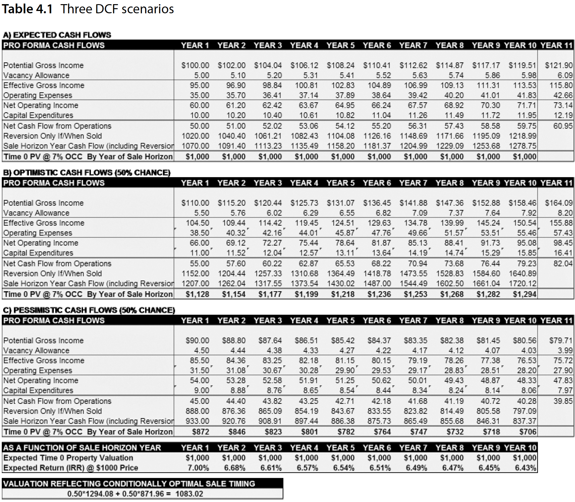
Specifically, we will be recreating the three DCF Scenarios in Table 4.1:
Again we import the necessary libraries:
import locale
import pandas as pd

import rangekeeper as rk
Base Parameters#
First let’s set up the Proforma Model’s parameters. These will be formatted as a dictionary of inputs:
locale.setlocale(locale.LC_ALL, 'en_AU')
units = rk.measure.Index.registry
currency = rk.measure.register_currency(registry=units)
params = {
    'start_date': pd.Timestamp('2001-01-01'),
    'num_periods': 10,
    'frequency': rk.duration.Type.YEAR,
    'acquisition_cost': -1000 * currency.units,
    'initial_income': 100 * currency.units,
    'growth_rate': 0.02,
    'vacancy_rate': 0.05,
    'opex_pgi_ratio': 0.35,
    'capex_pgi_ratio': 0.1,
    'exit_caprate': 0.05,
    'discount_rate': 0.07,

    # Table 4.1 has proformas that absorb an additional straight-line income flow:
    'addl_pgi_init': 0,
    'addl_pgi_slope': 0,
    }
Base Proforma Model#
Then let’s set up the base proforma model, which will accept the dict of
parameters on initialization:
class Model:
    def __init__(self, params: dict):
        self.params = params
In order to make the class more readable, we will use the @rk.update_class
decorator in order to sequentially add methods to the class in the following
cells. This is not necessary, but it helps when the documentation is in Jupyter
format.
Spans#
First we set up the Model’s Spans:
@rk.update_class(Model)
class Model:
    def init_spans(self):
        self.calc_span = rk.duration.Span.from_duration(
            name='Span to Calculate Reversion',
            date=self.params['start_date'],
            duration=self.params['frequency'],
            amount=self.params['num_periods'] + 1)
        self.acq_span = rk.duration.Span.from_duration(
            name='Acquisition Span',
            date=rk.duration.offset(
                self.params['start_date'],
                amount=-1,
                duration=self.params['frequency']),
            duration=self.params['frequency']
            )
        self.span = self.calc_span.extend(
            name='Span',
            amount=-1,
            duration=self.params['frequency'],
            bound='end')
Cash Flows#
We now set up the Model’s Operational Cash Flows:
@rk.update_class(Model)
class Model:
    def init_flows(self):
        self.acquisition = rk.flux.Flow.from_projection(
            name='Acquisition',
            value=self.params['acquisition_cost'],
            proj=rk.projection.Distribution(
                form=rk.distribution.Uniform(),
                sequence=self.acq_span.to_sequence(frequency=self.params['frequency'])),
            units=currency.units)

        self.base_pgi = rk.flux.Flow.from_projection(
            name='Base Potential Gross Income',
            value=self.params['initial_income'],
            proj=rk.projection.Extrapolation(
            form=rk.extrapolation.Compounding(
                rate=self.params['growth_rate']),
            sequence=self.calc_span.to_sequence(frequency=self.params['frequency'])),
            units=currency.units)

        # Table 4.1 has proformas that absorb an additional straight-line income
        # flow:
        self.addl_pgi = rk.flux.Flow.from_projection(
            name='Additional Potential Gross Income',
            value=self.params['addl_pgi_init'],
            proj=rk.projection.Extrapolation(
                form=rk.extrapolation.StraightLine(
                    slope=self.params['addl_pgi_slope']),
                sequence=self.calc_span.to_sequence(frequency=self.params['frequency'])),
            units=currency.units)

        self.pgi = (rk.flux.Stream(
            name='Potential Gross Income',
            flows=[self.base_pgi, self.addl_pgi],
            frequency=self.params['frequency'])
                .sum())

        self.vacancy = rk.flux.Flow(
            name='Vacancy Allowance',
            movements=self.pgi.movements * -self.params['vacancy_rate'],
            units=currency.units)
        self.egi = (rk.flux.Stream(
            name='Effective Gross Income',
            flows=[self.pgi, self.vacancy],
            frequency=self.params['frequency'])
                .sum())
        self.opex = (rk.flux.Flow(
            name='Operating Expenses',
            movements=self.pgi.movements * self.params['opex_pgi_ratio'],
            units=currency.units)
                .negate())
        self.noi = (rk.flux.Stream(
            name='Net Operating Income',
            flows=[self.egi, self.opex],
            frequency=self.params['frequency'])
                .sum())
        self.capex = rk.flux.Flow(
            name='Capital Expenditures',
            movements=self.pgi.movements * self.params['capex_pgi_ratio'],
            units=currency.units).negate()
        self.net_cfs = (rk.flux.Stream(
            name='Net Annual Cashflows',
            flows=[self.noi, self.capex],
            frequency=self.params['frequency'])
                .sum())

        self.reversions = rk.flux.Flow(
            name='Reversions',
            movements=self.net_cfs.movements.shift(periods=-1).dropna() / self.params['exit_caprate'],
            units=currency.units).trim_to_span(span=self.span)
        self.net_cfs = self.net_cfs.trim_to_span(span=self.span)
Metrics#
Now we can add methods to calculate metrics, like the present value (PV) and
internal rate of return (IRR) for each period in the Model’s Span:
@rk.update_class(Model)
class Model:
    def calc_metrics(self):
        pvs = []
        irrs = []
        for period in self.net_cfs.movements.index:
            cumulative_net_cfs = self.net_cfs.trim_to_span(
                span=rk.duration.Span(
                    name='Cumulative Net Cashflow Span',
                    start_date=self.params['start_date'],
                    end_date=period))
            reversion = rk.flux.Flow(
                movements=self.reversions.movements.loc[[period]],
                units=currency.units)
            cumulative_net_cfs_with_rev = rk.flux.Stream(
                name='Net Cashflow with Reversion',
                flows=[cumulative_net_cfs, reversion],
                frequency=self.params['frequency'])
            pv = (cumulative_net_cfs_with_rev
                .sum()
                .pv(
                    name='Present Value',
                    frequency=self.params['frequency'],
                    rate=self.params['discount_rate'])
                )
            pvs.append(pv.collapse().movements)

            incl_acq = rk.flux.Stream(
                name='Net Cashflow with Reversion and Acquisition',
                flows=[cumulative_net_cfs_with_rev.sum(), self.acquisition],
                frequency=self.params['frequency'])

            irrs.append(round(incl_acq.sum().irr(), 4))

        self.pvs = rk.flux.Flow(
            name='Present Values',
            movements=pd.concat(pvs),
            units=currency.units)
        self.irrs = rk.flux.Flow(
            name='Internal Rates of Return',
            movements=pd.Series(irrs, index=self.pvs.movements.index),
            units=None)
Output#
Now our Proforma Model is set up, and we can initialize and calculate it:
model = Model(params)
model.init_spans()
model.init_flows()
model.calc_metrics()
model.pvs
| date | Present Values |
|---|---|
| 2001-12-31 00:00:00 | $1,000.00 |
| 2002-12-31 00:00:00 | $1,000.00 |
| 2003-12-31 00:00:00 | $1,000.00 |
| 2004-12-31 00:00:00 | $1,000.00 |
| 2005-12-31 00:00:00 | $1,000.00 |
| 2006-12-31 00:00:00 | $1,000.00 |
| 2007-12-31 00:00:00 | $1,000.00 |
| 2008-12-31 00:00:00 | $1,000.00 |
| 2009-12-31 00:00:00 | $1,000.00 |
| 2010-12-31 00:00:00 | $1,000.00 |
model.irrs
| date | Internal Rates of Return |
|---|---|
| 2001-12-31 00:00:00 | 0.07 |
| 2002-12-31 00:00:00 | 0.07 |
| 2003-12-31 00:00:00 | 0.07 |
| 2004-12-31 00:00:00 | 0.07 |
| 2005-12-31 00:00:00 | 0.07 |
| 2006-12-31 00:00:00 | 0.07 |
| 2007-12-31 00:00:00 | 0.07 |
| 2008-12-31 00:00:00 | 0.07 |
| 2009-12-31 00:00:00 | 0.07 |
| 2010-12-31 00:00:00 | 0.07 |
Scenarios#
Optimistic#
In Table 4.1, the ‘Panel B’ (Optimistic) scenario is created by increasing the
initial income Flow by 10%, and also adding additional Potential Gross Income
with a Projection that compounds at 3% p.a.:
optimistic_params = params.copy()
optimistic_params['initial_income'] = params['initial_income'] + 10 * currency.units
optimistic_params['addl_pgi_slope'] = 3
Again, we can create a new Model with these parameters, and calculate it:
optimistic = Model(optimistic_params)
optimistic.init_spans()
optimistic.init_flows()
optimistic.calc_metrics()
optimistic.pvs
| date | Present Values |
|---|---|
| 2001-12-31 00:00:00 | $1,128.04 |
| 2002-12-31 00:00:00 | $1,153.72 |
| 2003-12-31 00:00:00 | $1,177.23 |
| 2004-12-31 00:00:00 | $1,198.74 |
| 2005-12-31 00:00:00 | $1,218.42 |
| 2006-12-31 00:00:00 | $1,236.41 |
| 2007-12-31 00:00:00 | $1,252.85 |
| 2008-12-31 00:00:00 | $1,267.87 |
| 2009-12-31 00:00:00 | $1,281.57 |
| 2010-12-31 00:00:00 | $1,294.08 |
optimistic.irrs
| date | Internal Rates of Return |
|---|---|
| 2001-12-31 00:00:00 | 0.21 |
| 2002-12-31 00:00:00 | 0.15 |
| 2003-12-31 00:00:00 | 0.13 |
| 2004-12-31 00:00:00 | 0.12 |
| 2005-12-31 00:00:00 | 0.12 |
| 2006-12-31 00:00:00 | 0.11 |
| 2007-12-31 00:00:00 | 0.11 |
| 2008-12-31 00:00:00 | 0.11 |
| 2009-12-31 00:00:00 | 0.11 |
| 2010-12-31 00:00:00 | 0.1 |
Pessimistic#
Similarly, we can create the ‘Panel C’ (Pessimistic) scenario:
pessimistic_params = params.copy()
pessimistic_params['initial_income'] = params['initial_income'] - 10 * currency.units
pessimistic_params['addl_pgi_slope'] = -3

pessimistic = Model(pessimistic_params)
pessimistic.init_spans()
pessimistic.init_flows()
pessimistic.calc_metrics()
pessimistic.pvs
| date | Present Values |
|---|---|
| 2001-12-31 00:00:00 | $871.96 |
| 2002-12-31 00:00:00 | $846.28 |
| 2003-12-31 00:00:00 | $822.77 |
| 2004-12-31 00:00:00 | $801.26 |
| 2005-12-31 00:00:00 | $781.58 |
| 2006-12-31 00:00:00 | $763.59 |
| 2007-12-31 00:00:00 | $747.15 |
| 2008-12-31 00:00:00 | $732.13 |
| 2009-12-31 00:00:00 | $718.43 |
| 2010-12-31 00:00:00 | $705.92 |
pessimistic.irrs
| date | Internal Rates of Return |
|---|---|
| 2001-12-31 00:00:00 | -0.07 |
| 2002-12-31 00:00:00 | -0.02 |
| 2003-12-31 00:00:00 | -0 |
| 2004-12-31 00:00:00 | 0.01 |
| 2005-12-31 00:00:00 | 0.01 |
| 2006-12-31 00:00:00 | 0.02 |
| 2007-12-31 00:00:00 | 0.02 |
| 2008-12-31 00:00:00 | 0.02 |
| 2009-12-31 00:00:00 | 0.02 |
| 2010-12-31 00:00:00 | 0.02 |
Analysis and Expected Value (EV)#
[dNG18] Table 4.1 continues with calculating the Expected Value (EV) of the outcome, given that both optimistic and pessimistic scenarios have a 50% chance of occuring:
# Expected Time 0 Property Valuation:
evs = (optimistic.pvs.movements + pessimistic.pvs.movements) / 2
evs
date
2001-12-31    1000.0
2002-12-31    1000.0
2003-12-31    1000.0
2004-12-31    1000.0
2005-12-31    1000.0
2006-12-31    1000.0
2007-12-31    1000.0
2008-12-31    1000.0
2009-12-31    1000.0
2010-12-31    1000.0
Name: Present Values, dtype: float64
And the expected return (IRR) at each time period is:
# Expected Return (IRR) at $1000 Price:
ers = (optimistic.irrs.movements + pessimistic.irrs.movements) / 2
ers
date
2001-12-31    0.070000
2002-12-31    0.066784
2003-12-31    0.066067
2004-12-31    0.065631
2005-12-31    0.065342
2006-12-31    0.065093
2007-12-31    0.064872
2008-12-31    0.064653
2009-12-31    0.064473
2010-12-31    0.064310
Name: Internal Rates of Return, dtype: float64
As documented in [dNG18] Chapter 4.3, we can calculate the value of the flexibility, assuming it is possible to sell the property at will:
# Valuation of Flexibility to Sell at Optimal Time:
value_of_flex = (optimistic.pvs.movements.iloc[-1] / 2 + pessimistic.pvs.movements.iloc[0] / 2) - evs.iloc[-1]
print("Value of flexiblity: ${:,.2f}".format(value_of_flex))
Value of flexiblity: $83.02