
Introduction to Modeling Flexibility#
Introducing flexibility into a Proforma allows for the modeling of decision points and alternate courses of action, which have optionality (the agency but not the requirement to act). This offers a more sophisticated, and realistic, simulation of real estate investment scenarios.
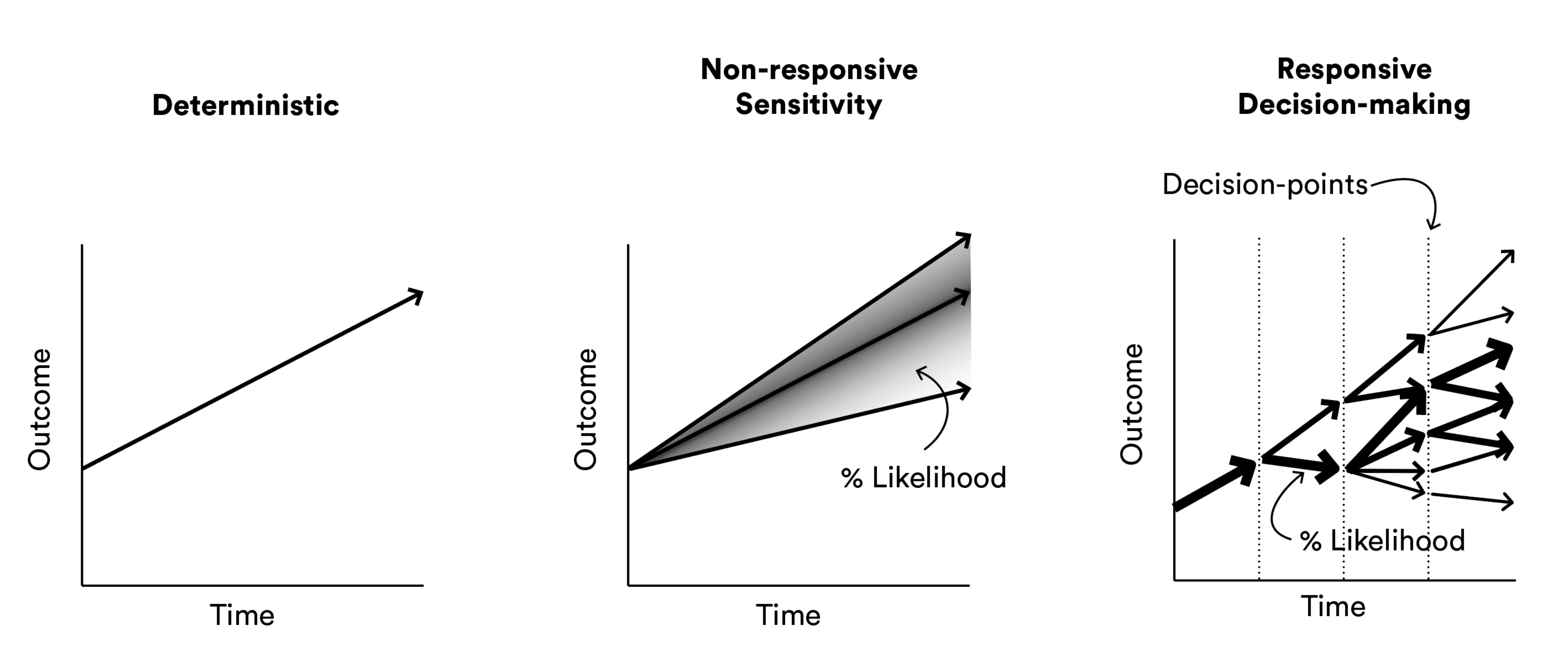
Fig. 4 How a basic Proforma can be progressed from simple deterministic projections, to non-responsive sensitivity analysis, to responsive decision-making.#
[dNG18] apply flexibility to a basic Proforma in two steps:
Using a simulated
Market’s pricing factors to adjust projected values for cash flows (by multiplying the factor against respective line items).Programming ‘decisions’ into the Proforma that change how the Proforma operates, in response to conditions or characteristics of the
Marketdynamics.
To begin with, let’s see how Rangekeeper adjusts the projected Potential Gross
Income and Reversion cash flows, using a single scenario/trial of a Market.
Similar to the Deterministic Scenario Analysis , we import required libraries and set up a base Model:
import locale
from typing import List

import warnings
warnings.filterwarnings("ignore")
import pandas as pd

import rangekeeper as rk
locale.setlocale(locale.LC_ALL, 'en_AU')
units = rk.measure.Index.registry
currency = rk.measure.register_currency(registry=units)
params = {
    'start_date': pd.Timestamp('2001-01-01'),
    'num_periods': 10,
    'frequency': rk.duration.Type.YEAR,
    'acquisition_cost': -1000 * currency.units,
    'initial_income': 100 * currency.units,
    'growth_rate': 0.02,
    'vacancy_rate': 0.05,
    'opex_pgi_ratio': 0.35,
    'capex_pgi_ratio': 0.1,
    'exit_caprate': 0.05,
    'discount_rate': 0.07
    }
Base (Ex-Ante, Inflexible) Model#
The Base (non-market-adjusted and inflexible) Model is the same as before:
class BaseModel:
    def __init__(self) -> None:
        pass

    def set_params(self, params: dict) -> None:
        self.params = params
Define Spans
Define Calculations for Cash Flows
Define Metrics
Wrap all definitions and calculations in a execute() method:
@rk.update_class(BaseModel)
class BaseModel:
    def generate(self):
        self.init_spans()
        self.calc_acquisition()
        self.calc_egi()
        self.calc_noi()
        self.calc_ncf()
        self.calc_reversion()
        self.calc_metrics()
This results in the ‘Ex-Ante Realistic Traditional DCF Proforma’:
ex_ante = BaseModel()
ex_ante.set_params(params)
ex_ante.generate()
ex_ante_table = rk.flux.Stream(
    name='Ex-Ante Pro-forma Cash Flow Projection',
    flows=[
        ex_ante.pgi,
        ex_ante.vacancy,
        ex_ante.egi,
        ex_ante.opex,
        ex_ante.noi,
        ex_ante.capex,
        ex_ante.net_cf,
        ex_ante.reversion,
        ],
    frequency=rk.duration.Type.YEAR
    )
ex_ante_table
| Potential Gross Income | Vacancy Allowance | Effective Gross Income (sum) | Operating Expenses | Net Operating Income (sum) | Capital Expenditures | Net Annual Cashflow (sum) | Reversion | |
|---|---|---|---|---|---|---|---|---|
| 2001 | $100.00 | -$5.00 | $95.00 | -$35.00 | $60.00 | -$10.00 | $50.00 | 0 |
| 2002 | $102.00 | -$5.10 | $96.90 | -$35.70 | $61.20 | -$10.20 | $51.00 | 0 |
| 2003 | $104.04 | -$5.20 | $98.84 | -$36.41 | $62.42 | -$10.40 | $52.02 | 0 |
| 2004 | $106.12 | -$5.31 | $100.81 | -$37.14 | $63.67 | -$10.61 | $53.06 | 0 |
| 2005 | $108.24 | -$5.41 | $102.83 | -$37.89 | $64.95 | -$10.82 | $54.12 | 0 |
| 2006 | $110.41 | -$5.52 | $104.89 | -$38.64 | $66.24 | -$11.04 | $55.20 | 0 |
| 2007 | $112.62 | -$5.63 | $106.99 | -$39.42 | $67.57 | -$11.26 | $56.31 | 0 |
| 2008 | $114.87 | -$5.74 | $109.13 | -$40.20 | $68.92 | -$11.49 | $57.43 | 0 |
| 2009 | $117.17 | -$5.86 | $111.31 | -$41.01 | $70.30 | -$11.72 | $58.58 | 0 |
| 2010 | $119.51 | -$5.98 | $113.53 | -$41.83 | $71.71 | -$11.95 | $59.75 | $1,218.99 |
| 2011 | $121.90 | -$6.09 | $115.80 | -$42.66 | $73.14 | -$12.19 | $60.95 | 0 |
The metrics for the Base Model are:
print('Projected IRR at Market Value Price: {:.2%}'.format(ex_ante.irrs.movements.iloc[-1]))
print('Time 0 Present Value at OCC: {0}'.format(locale.currency(ex_ante.pvs.movements.iloc[-1], grouping=True)))
print('Average Annual Cashflow: {0}'.format(locale.currency(ex_ante.net_cf.trim_to_span(ex_ante.span).movements.mean(), grouping=True)))
Projected IRR at Market Value Price: 7.00%
Time 0 Present Value at OCC: $1,000.00
Average Annual Cashflow: $54.75
Warning
Note that the holding period for the Base Model is fixed (inflexible) at 10 years.
Note
The Average Annual Cashflow is derived from the Operating cash flow only (not counting reversion). This is to indicate the relative favorability of the scenario outcomes in terms of the real estate space market, the fundamental economic basis of the property value.
(From [dNG18], accompanying Excel spreadsheets)
Ex-Post Inflexible Model#
The Ex-Post Model uses a simulated Market scenario to adjust the Base
Model’s Potential Gross Income (PGI) and Reversion cash flows. In this case,
instead of using straight-line projected growth to calculate the PGI, we will
use the simulated Market’s Price Factors to adjust the Ex-Ante Model (and
emulate how an ‘Ex-Post’ Model would look)
Market#
First, we need to simulate a Market scenario:
frequency = rk.duration.Type.YEAR
num_periods = 25
span = rk.duration.Span.from_duration(
    name="Span",
    date=pd.Timestamp(2000, 1, 1),
    duration=frequency,
    amount=num_periods)
sequence = span.to_sequence(frequency=frequency)
Overall Trend:
trend = rk.dynamics.trend.Trend(
    sequence=sequence,
    cap_rate=.05,
    initial_value=0.050747414,
    growth_rate=-0.002537905)
Volatility:
volatility = rk.dynamics.volatility.Volatility(
    sequence=sequence,
    trend=trend,
    volatility_per_period=.1,
    autoregression_param=.2,
    mean_reversion_param=.3)
Cyclicality:
cyclicality = rk.dynamics.cyclicality.Cyclicality.from_estimates(
    space_cycle_phase_prop=0,
    space_cycle_period=13.8,
    space_cycle_height=1,
    space_cycle_asymmetric_parameter=.5,
    asset_cycle_period_diff=0.8,
    asset_cycle_phase_diff_prop=-.05,
    asset_cycle_amplitude=.02,
    asset_cycle_asymmetric_parameter=.5,
    sequence=sequence)
Noise and Black Swan:
noise = rk.dynamics.noise.Noise(
    sequence=sequence,
    noise_dist=rk.distribution.Symmetric(
        type=rk.distribution.Type.TRIANGULAR,
        residual=.1))

black_swan = rk.dynamics.black_swan.BlackSwan(
    sequence=sequence,
    likelihood=.05,
    dissipation_rate=.3,
    probability=rk.distribution.Uniform(),
    impact=-.25)
Single Market Scenario:
market = rk.dynamics.market.Market(
    sequence=sequence,
    trend=trend,
    volatility=volatility,
    cyclicality=cyclicality,
    noise=noise,
    black_swan=black_swan)
table = rk.flux.Stream(
    name='Market Dynamics',
    flows=[
        market.trend,
        market.volatility.volatility,
        market.volatility.autoregressive_returns,
        market.volatility,
        market.cyclicality.space_waveform,
        market.space_market,
        market.cyclicality.asset_waveform,
        market.asset_market,
        market.asset_true_value,
        market.space_market_price_factors,
        market.noisy_value,
        market.historical_value,
        market.implied_rev_cap_rate,
        market.returns
        ],
    frequency=frequency)
table.plot(
        flows={
            'Market Trend': (0, .1),
            'Space Market': (0, .1),
            'Historical Value': (0, 3)
            }
        )
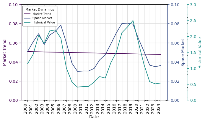
Warning
Note where market peaks and troughs are!
Model#
Now we can duplicate and edit (subclass) the Base Model to create the Inflexible Ex-Post Model.
class ExPostInflexModel(BaseModel):
    def set_market(self, market: rk.dynamics.market.Market) -> None:
        self.market = market
In order to use the simulated Market’s Space Market Price Factors to adjust
the Base Model’s PGI, we need to override the calc_egi() method and instead
calculate the product of a Stream object whose two Flows are the Base
Model’s PGI and the simulated Market’s Space Market Price Factors:
@rk.update_class(ExPostInflexModel)
class ExPostInflexModel(BaseModel):
    def calc_egi(self):
        pgi = rk.flux.Flow.from_projection(
            name='Potential Gross Income',
            value=self.params['initial_income'],
            proj=rk.projection.Extrapolation(
                form=rk.extrapolation.Compounding(
                    rate=self.params['growth_rate']),
                sequence=self.calc_span.to_sequence(frequency=self.params['frequency'])),
            units=currency.units)

        # Construct a Stream that multiplies the Base Model's PGI by the
        # simulated Market's Space Market factors
        self.pgi = (rk.flux.Stream(
            name='Potential Gross Income',
            flows=[
                pgi,
                self.market.space_market_price_factors.trim_to_span(self.calc_span)
                ],
            frequency=self.params['frequency'])
                .product(registry=rk.measure.Index.registry))

        self.vacancy = rk.flux.Flow(
            name='Vacancy Allowance',
            movements=self.pgi.movements * -self.params['vacancy_rate'],
            units=currency.units)
        self.egi = (rk.flux.Stream(
            name='Effective Gross Income',
            flows=[
                self.pgi,
                self.vacancy
                ],
            frequency=self.params['frequency'])
                .sum())
Similarly, we override the calc_reversion() method to use the simulated
Market’s implied reversion cap rates to calculate the Reversions:
@rk.update_class(ExPostInflexModel)
class ExPostInflexModel(BaseModel):
    def calc_reversion(self):
        # Construct the Reversions using the simulated Market's Asset Market
        # factors (cap rates):
        self.reversions = (rk.flux.Flow(
            name='Reversions',
            movements=self.net_cf.movements.shift(periods=-1).dropna() /
                      self.market.implied_rev_cap_rate.movements,
            units=currency.units)
                .trim_to_span(span=self.span))

        self.reversion = self.reversions.trim_to_span(
            span=self.reversion_span,
            name='Reversion')
        self.pbtcfs = rk.flux.Stream(
            name='PBTCFs',
            flows=[
                self.net_cf.trim_to_span(span=self.span),
                self.reversions.trim_to_span(span=self.reversion_span)
                ],
            frequency=self.params['frequency'])
Copy the parameters and execute the model:
ex_post_params = params.copy()
ex_post_inflex = ExPostInflexModel()
ex_post_inflex.set_params(ex_post_params)
ex_post_inflex.set_market(market)
ex_post_inflex.generate()
ex_post_table = rk.flux.Stream(
    name='Ex-Ante Pro-forma Cash Flow Projection',
    flows=[
        ex_post_inflex.pgi,
        ex_post_inflex.vacancy,
        ex_post_inflex.egi,
        ex_post_inflex.opex,
        ex_post_inflex.noi,
        ex_post_inflex.capex,
        ex_post_inflex.net_cf,
        ex_post_inflex.reversion,
        ],
    frequency=rk.duration.Type.YEAR
    )
ex_post_table
| Potential Gross Income (product) | Vacancy Allowance | Effective Gross Income (sum) | Operating Expenses | Net Operating Income (sum) | Capital Expenditures | Net Annual Cashflow (sum) | Reversion | |
|---|---|---|---|---|---|---|---|---|
| 2001 | $119.90 | -$5.99 | $113.90 | -$41.96 | $71.94 | -$11.99 | $59.95 | 0 |
| 2002 | $139.48 | -$6.97 | $132.50 | -$48.82 | $83.69 | -$13.95 | $69.74 | 0 |
| 2003 | $119.13 | -$5.96 | $113.18 | -$41.70 | $71.48 | -$11.91 | $59.57 | 0 |
| 2004 | $142.21 | -$7.11 | $135.10 | -$49.78 | $85.33 | -$14.22 | $71.11 | 0 |
| 2005 | $153.18 | -$7.66 | $145.52 | -$53.61 | $91.91 | -$15.32 | $76.59 | 0 |
| 2006 | $170.25 | -$8.51 | $161.74 | -$59.59 | $102.15 | -$17.02 | $85.12 | 0 |
| 2007 | $133.01 | -$6.65 | $126.36 | -$46.55 | $79.80 | -$13.30 | $66.50 | 0 |
| 2008 | $87.31 | -$4.37 | $82.94 | -$30.56 | $52.38 | -$8.73 | $43.65 | 0 |
| 2009 | $69.17 | -$3.46 | $65.71 | -$24.21 | $41.50 | -$6.92 | $34.58 | 0 |
| 2010 | $71.78 | -$3.59 | $68.20 | -$25.12 | $43.07 | -$7.18 | $35.89 | $512.81 |
| 2011 | $73.17 | -$3.66 | $69.51 | -$25.61 | $43.90 | -$7.32 | $36.59 | 0 |
We can compare models on the same metrics:
print('Projected IRR at Market Value Price: {:.2%}'.format(ex_post_inflex.irrs.movements.iloc[-1]))
print('Time 0 Present Value at OCC: {0}'.format(locale.currency(ex_post_inflex.pvs.movements.iloc[-1], grouping=True)))
print('Average Annual Cashflow: {0}'.format(locale.currency(ex_post_inflex.net_cf.trim_to_span(ex_post_inflex.span).movements.mean(), grouping=True)))
Projected IRR at Market Value Price: 1.52%
Time 0 Present Value at OCC: $695.70
Average Annual Cashflow: $60.27
pv_diff = (ex_post_inflex.pvs.movements.iloc[-1] - ex_ante.pvs.movements.iloc[-1]) / ex_ante.pvs.movements.iloc[-1]
print('Percentage Difference of Scenario PV Minus Pro-forma PV: {:.2%}'.format(pv_diff))

irr_diff = ex_post_inflex.irrs.movements.iloc[-1] - ex_ante.irrs.movements.iloc[-1]
print('Difference of Scenario IRR Minus Pro-forma IRR: {:.2%}'.format(irr_diff))
Percentage Difference of Scenario PV Minus Pro-forma PV: -30.43%
Difference of Scenario IRR Minus Pro-forma IRR: -5.48%
Ex-Post Flexible Model#
In attempting to capture the effects of flexibility in our Proforma, we must introduce the ability to program optionality into our model; that is, the creation of alternate options to a single course of action, that may be exercised (but are not obliged to be)
In [dNG18], Chapter 9 presents a simple case of flexibility; the ‘Resale Timing Problem’, which is described as the question of when and how to decide to sell an investment property.
Rangekeeper formulates these types of decision problems as Policys that
encapsulate the sequence of conditions required to trigger a decision, and the
option actions that are execised as a result.
Policys#
Policys adjust or edit a Model dynamically (e.g. by overwriting how it
constructs its Flows, Streams, or metrics/outcomes), and thus enable the
Proforma to be flexible.
They are structured as classes that require a ‘state’ (a specific Flow) to be
checked for a certain ‘condition’, and if the condition is met, an ‘action’ on
the Model is executed; producing a new Model.
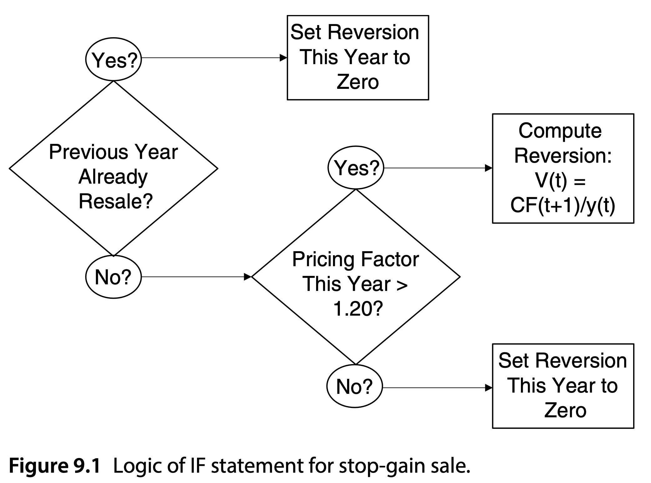
[dNG18] diagram the logic of the “Stop-Gain Resale Rule” as a flowchart (influenced by Excel functions). In Rangekeeper, this would be programmed as simply adjusting the holding period of the asset (in effect bringing its reversion/sale to the specified period):
First we define our condition, taking a Flow as input and outputting a
sequence of respective booleans that flag the state of the decision.
Note
Note an additional condition has been specified in the below code; that the
minimum hold period is 7 years. This is to prevent the model from triggering
consistently in the first few years as the Market phase has been fixed at ‘0’
(ie, the scenario always begins with a Market at mid-cycle going up)
def exceed_pricing_factor(state: rk.flux.Flow) -> List[bool]:
    threshold = 1.2
    result = []
    for i in range(state.movements.index.size):
        if any(result):
            result.append(False)
        else:
            if i < 7:
                result.append(False)
            else:
                if state.movements.iloc[i] > threshold:
                    result.append(True)
                else:
                    result.append(False)
    return result
Now we define our action; taking a Model object to manipulate, as well as the
resultant sequence of decisions from the previous condition check:
def adjust_hold_period(
        model: object,
        decisions: List[bool]) -> object:
    # Get the index of the decision flag:
    try:
        idx = decisions.index(True)
    except ValueError:
        idx = len(decisions)

    # Adjust the Model's holding period:
    policy_params = model.params.copy()
    policy_params['num_periods'] = idx

    # Re-run the Model with updated params:
    model.set_params(policy_params)
    model.generate()
    return model
Now that our functions have been defined, we wrap them in a Policy instance,
that can be executed against the Model and its context (Market)
Note
The abstract nature of the Policy class implies the ability to chain multiple
Policys together, thus building more complex graphs of actions that can better
mimic a manager or developer of a real estate asset. For more information, see
Markov decision process
stop_gain_resale_policy = rk.policy.Policy(
    condition=exceed_pricing_factor,
    action=adjust_hold_period)
ex_post_flex = stop_gain_resale_policy.execute(
    args=(ex_post_inflex.market.space_market_price_factors, ex_post_inflex))

print('Flexible Model Hold Period: {0}'.format(ex_post_flex.params['num_periods']))
print('Projected IRR at Market Value Price: {:.2%}'.format(ex_post_flex.irrs.movements.iloc[-1]))
print('Time 0 Present Value at OCC: {0}'.format(locale.currency(ex_post_flex.pvs.movements.iloc[-1], grouping=True)))
print('Average Annual Cashflow: {0}'.format(locale.currency(ex_post_flex.net_cf.trim_to_span(ex_post_inflex.span).movements.mean(), grouping=True)))
Flexible Model Hold Period: 16
Projected IRR at Market Value Price: 9.20%
Time 0 Present Value at OCC: $1,264.86
Average Annual Cashflow: $60.14
In this situation, flexibility is a benefit to the investor, as Stop-Gain Resale Policy encourages holding the asset until the market peaks, and avoids market downturns.